In this tutorial it is demonstrated how MATLAB can be used to create a drill cycle pattern which can be imported into IRBCAM as a CSV file. The tutorial is available inside IRBCAM as a Shared Project with the name TUTORIAL_MATLAB_DRILL
The MATLAB script generates a CSV file according to the Documentation
MATLAB is a very powerful platform with a large collection of different toolboxes. Advanced 5-axis (or even 6-axis) toolpaths can be generated in MATLAB for use in IRBCAM, as an alternative to creating the toolpaths using CAD/CAM software.
The MATLAB script used in this example is made available below:
clear;

% X range of drill pattern
xmin = 0; xmax = 1000; dx = 100;
% Y range of drill pattern
ymin = -1000; ymax = 1000; dy = 100;

% Constant variables
z = 50;
z_drill = 50;
rz1 = 0;
ry = pi;
rz2 = 0;
velocity = 100;  % Float (mm/s)
motion_type = 0; % Integer (Linear move)
tool_number = 1; % Integer
spindle = 1000;  % Float (extra data associated with tool)

data = [];
for(x = xmin:dx:xmax)
    for(y = ymin:dy:ymax)
        data = [data; x y z rz1 ry rz2 motion_type velocity tool_number spindle];
        data = [data; x y z-z_drill rz1 ry rz2 motion_type velocity tool_number spindle];
        data = [data; x y z rz1 ry rz2 motion_type velocity tool_number spindle];
    end
end

strHeader = 'x,y,z,rz1,ry,rz2,motion_type,velocity,tool_number,spindle_speed';
fid=fopen('data.csv','w');
fprintf(fid,'%s\n',strHeader);
fclose(fid);
writematrix(data,'data.csv','WriteMode','append');

plot3(data(:,1), data(:,2), data(:,3),'bo');
grid on;
title('Drill Pattern for IRBCAM Demo');
xlabel('X axis (mm)');
ylabel('Y axis (mm)');
If you run this Matlab script, the following figure will be displayed:
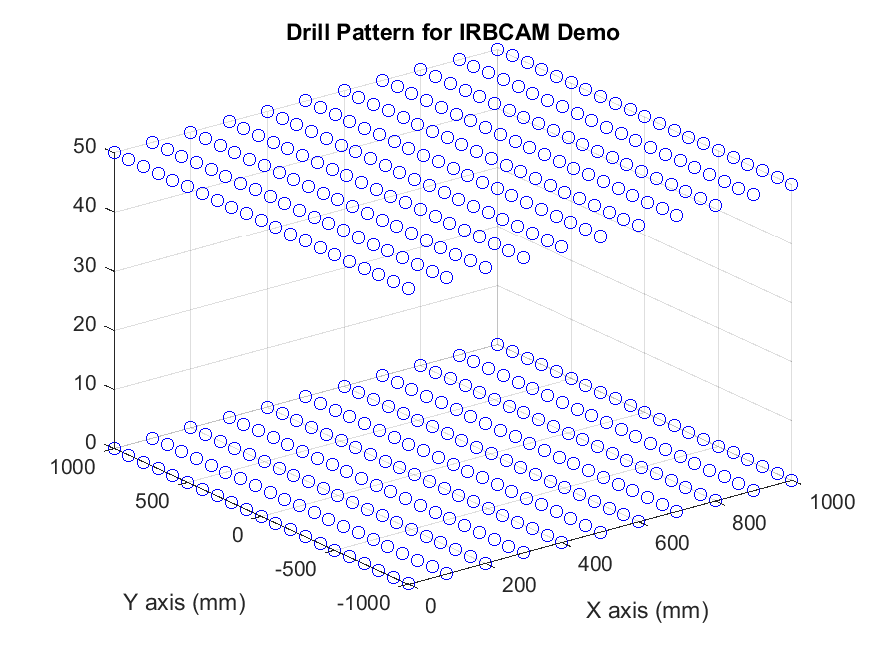
The generated data.csv file is made available at the bottom of this tutorial.
Start with an empty project in IRBCAM and load the robot FANUC-R2000iA-210F. Select the spindle tool ELTE-TMA4. Define the user frame at X=1500, Y=0 and Z=500.
Select Edit - Additional Objects - Cuboid and define the position as X=1500, Y=-1000, Z=0. Size X=1000, Y=2000, Z=500. Select a color, for example light blue.
Select View - Combination View. After that FIle - Import Path and select the CSV file generated by Matlab, data.csv.
A screenshot after these steps is shown below:
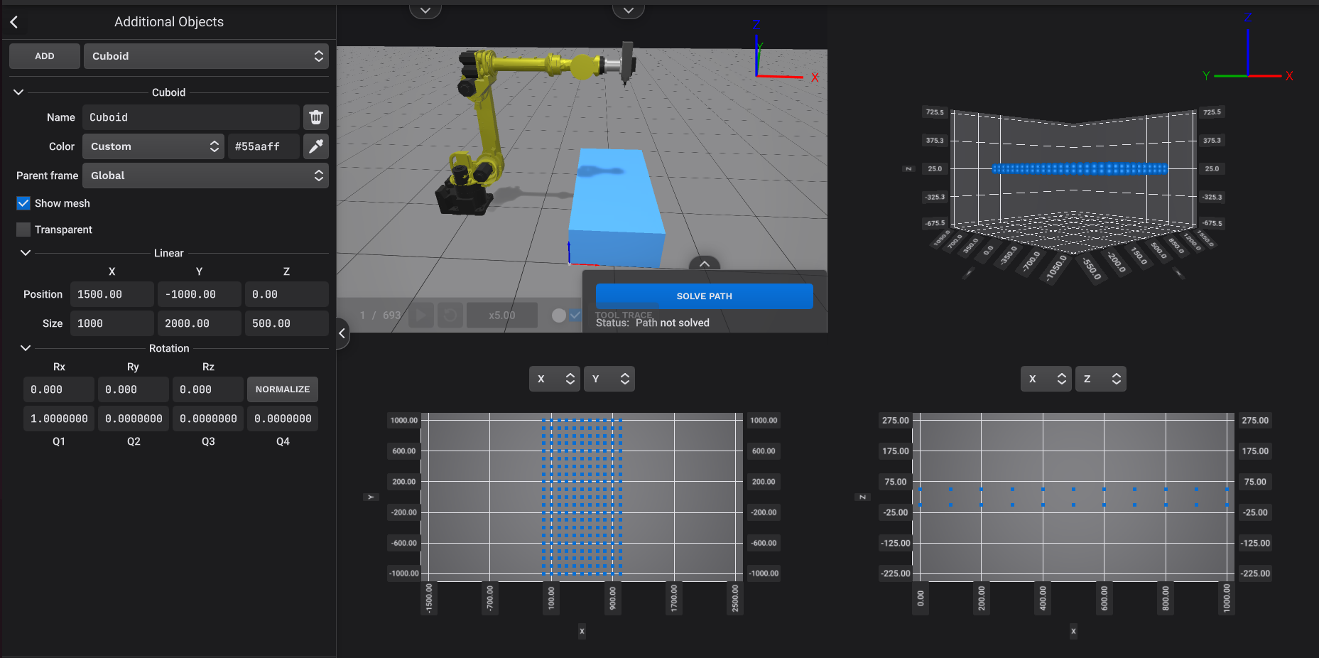
The drill cycle pattern is clearly visible in the XY plot, while the liftpoints are visible in the XZ plot.
Next, select View - Station and then go to Edit - Targets and select the first target. The robot will move into position with the default configuration settings.
In the bottom right corner of the IRBCAM window, you will find the parameters for the Solve Path function. Select the following parameters to solve and configure the robot’s path:
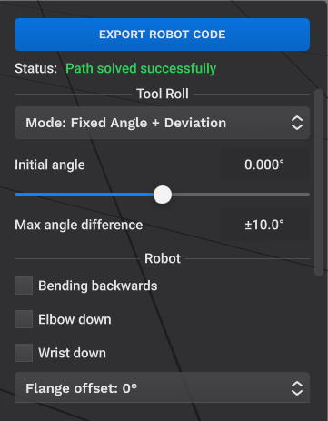
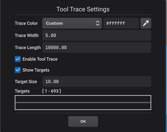
Click on TOOL TRACE and define the following parameters:
Next, increase the simulation speed by a factor x10 as shown below:
and press the Play icon. A video of this simulation is shown below:
data.zip (1.5 KB)