This tutorial is available inside IRBCAM as a shared project, with the name TUTORIAL_PYTHON_SPLINE. When selecting File - Open Project, look for this project under the section “Shared with me” near the bottom of the file open dialog window.
Most robot controllers do not support splines natively. Splines are useful when you want the robot to pass through the points with continuous velocities and accelerations, rather than just close to the points. This can be an advantage in robotic machining to reduce and minimize vibrations in the robot’s arm structure.
In this tutorial we demonstrate how to create a spline-interpolated toolpath from sample data and create a JSON file which can be imported into IRBCAM. The generated JSON data follows the format specified in the Documentation. The toolpath in this example is configured and simulated using a MOTOMAN-MH80 robot.
Python has a large number of advanced toolboxes, such as numpy and scipy. These can be used as an alternative to CAD/CAM software to create advanced 5-axis (or even 6-axis) robotics toolpaths which can be imported into IRBCAM.
The Python code to generate the spline interpolated JSON file is given below. To run the code, some packages are required: pip3 install numpy scipy matplotlib
import json
import numpy as np
import matplotlib.pyplot as plt
from scipy.interpolate import UnivariateSpline
from math import pi
# Vector lengths
L1 = 10 # Length of sample data
L2 = 100 # Length of smooth data
# Sample data points
x = np.linspace(0, 500, L1)
y = 100*np.sin(x) + 100*np.sin(x) ** 2 + 50*np.cos(x)
# Create a spline of the data
spline = UnivariateSpline(x, y)
# Generate finer points for a smooth curve
x_smooth = np.linspace(0, 500, L2)
y_smooth = spline(x_smooth)
# Generate JSON data for IRBCAM
data = \
{ \
"targets": { \
"pX": [], "pY": [], "pZ": [], "rZ": [], "rY": [], "rz2": [], "type": [] \
}, \
"velocity": {"i": [0], "value": [100]}, \
"tool": {"i": [0], "value": [1]}, \
"spindle": {"i": [0], "value": [1000]} \
}
data["targets"]["pX"] = x_smooth.tolist()
data["targets"]["pY"] = y_smooth.tolist()
data["targets"]["pZ"] = np.zeros(L2).tolist()
data["targets"]["rZ"] = np.zeros(L2).tolist()
data["targets"]["rY"] = (pi * np.ones(L2)).tolist()
data["targets"]["rz2"] = np.zeros(L2).tolist()
data["targets"]["type"] = [0] * L2
with open('spline.json', 'w') as f:
json.dump(data, f)
# Plotting the original data points and the spline
plt.figure(figsize=(8, 4))
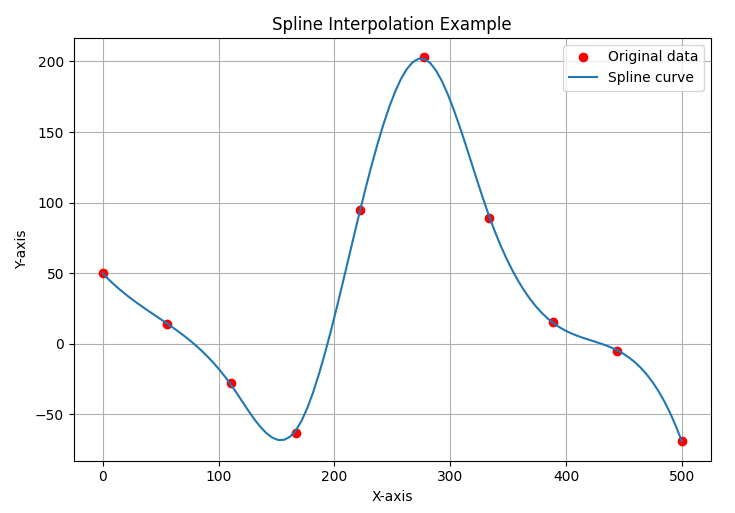
plt.plot(x, y, 'ro', label='Original data')
plt.plot(x_smooth, y_smooth, label='Spline curve')
plt.legend()
plt.title('Spline Interpolation Example')
plt.xlabel('X-axis')
plt.ylabel('Y-axis')
plt.grid(True)
plt.show()
When running this Python script, the following plot will be displayed:
and the file spline.json is generated. This file is made available for download at the bottom of this tutorial.
Start with an empty project and load the robot model MOTOMAN-MH80 with the tool ELTE-TMA4. Define the user frame at X=1500, Y=0 and Z=500 (millimeters). In this tutorial we are not using any user-defined objects. Go to File - Import Path and select spline.json.
Selevt View - Combination View and the screen should look similar to the one below:
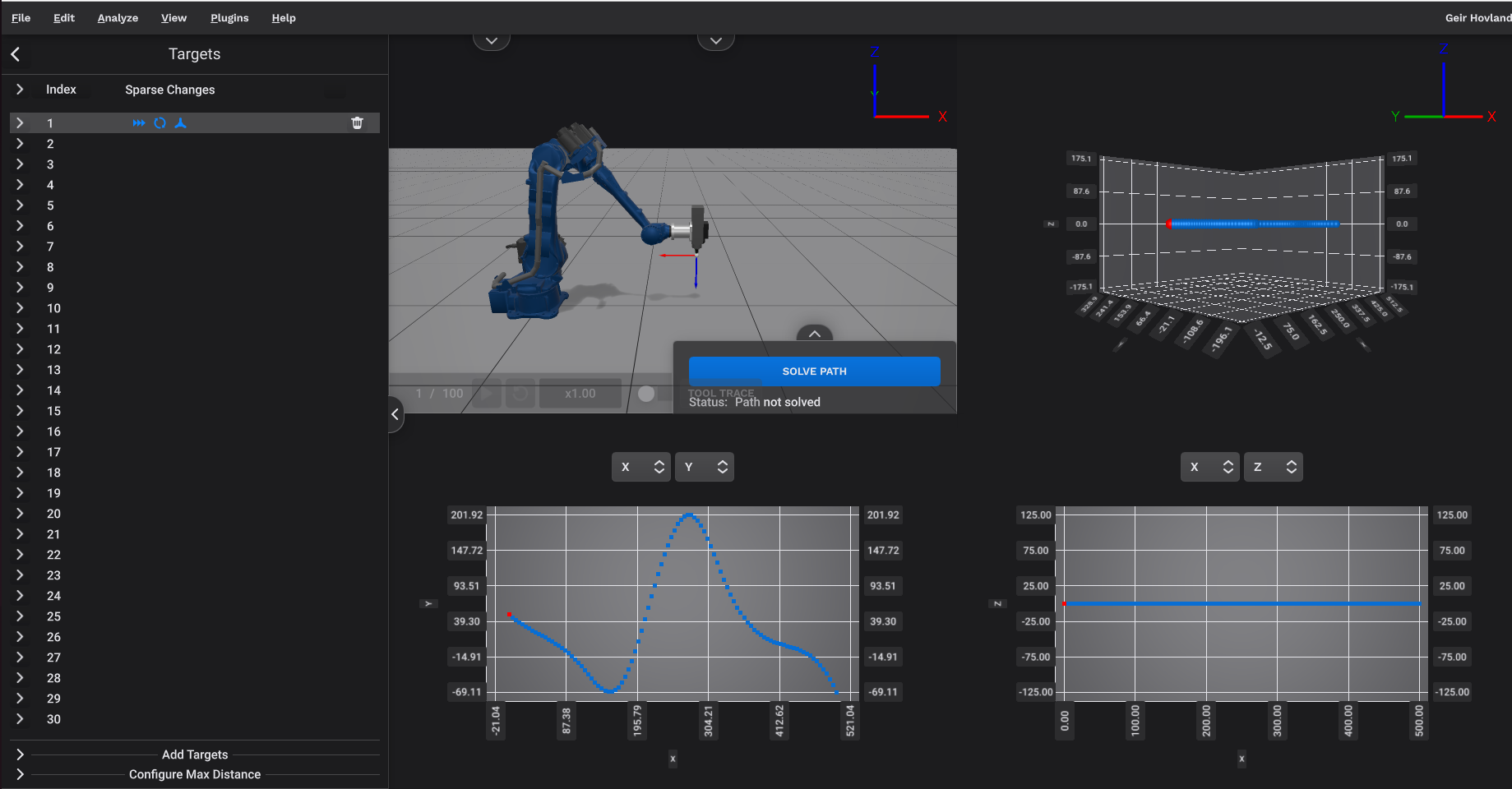
Notice that in the XY-plot the curve is the same as in the figure displayed by the Python script above.
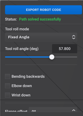
Select View - Station, then go to Edit - Targets and select target number 1. After that go to Solve Path and use the parameters shown below:
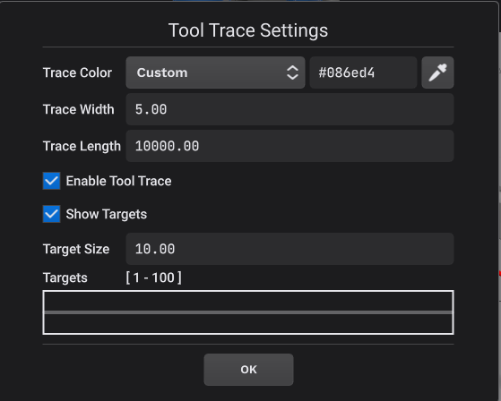
Select the Tool Trace parameters as shown below:
The robot with this toolpath can now be simulated by clicking on the Play icon, as shown in the movie below:
This tutorial has demonstrated how it is possible to create and configure a spline-interpolated toolpath even for robot controllers which do not natively support this feature. The accuracy of the final robot path can be controlled by how densely the interpolated points are generated in the Python script.
spline.zip (1.9 KB)