In this tutorial it will be demonstrated how to chain multiple toolpaths together and how to Solve Path when machining 5 sides of a cube. The APT files needed are made available at the bottom of this tutorial.
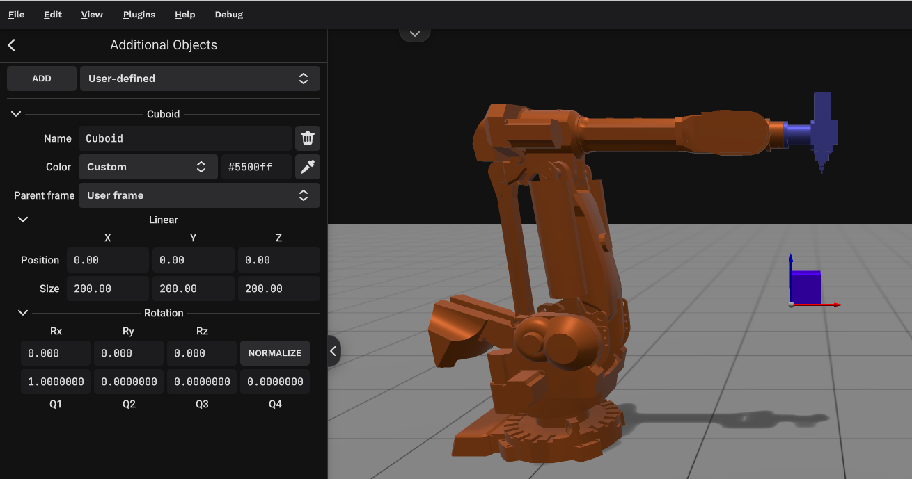
First, define a project with an ABB IRB6400R-2.5-200 robot and attach the spindle ELTE-TMA4 to it. Define the User Frame at X=1650, Y=0, Z=1000 and add an Additional Object - Cuboid with settings as shown below:
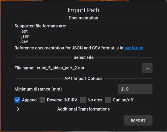
Next, import the APT file named cube_5_sides_part_1.apt. After this, import the second APT file named cube_5_sides_part_2.apt and mark the checkbox Append as seen below:
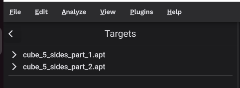
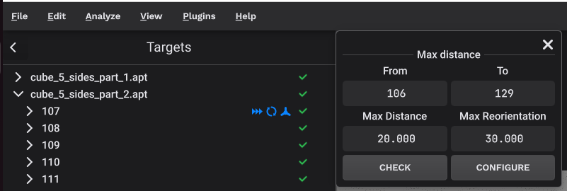
If there were more APT files to include, they can just be added sequentially with the Append option checked. When you go to Edit - View Targets, you can see that the two imported paths have been grouped separately:
When all APT files have been chained together into the station, select Edit - Targets and right-click on the first path, then select “Open max distance editor”. Use this function: click on CHECK then edit with the parameters seen below:
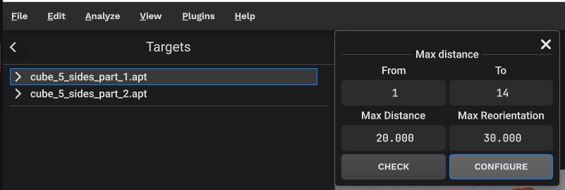
Finally click on CONFIGURE. What this function does is to interpolate the toolpath from the chained APT files with a maximum linear distance of 20mm and a maximum orientation change of 30 degrees between the targets. With smaller distances between the targets in both linear and orientation directions it will be easier for IRBCAM to solve the path and to reduce the risk of unwanted movements between the targets and collisions.
Right-click and configure the maximum distance also for the second path, but make the “From target” index equal to 106 instead of 107, to make sure that the transition between the two path groups is also included. See screenshot below:
After Configure Max Distance on both paths with the settings above, the number of targets will increase from 37 to 290.
In general, if you want to “stitch together” (or in other words, configure the transition between) two paths which are otherwise OK, you select the last target in the first path as “From” and the first target in the second path as “To” in the maximum distance editor, then CONFIGURE. Any new targets in such a case, will be added to the beginning of the second path, while the first one will remain unchanged.
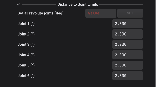
To make sure that we have an extra buffer distance to the joint limits in this example, we increase all the distances to the joint limits to 2.0 degrees, as shown below. These settings are found in the menu File - Settings - Station.
Finally, go to SOLVE PATH and use the settings shown below:
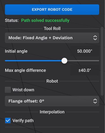
Note that Fixed Angle + Deviation is selected here with an initial tool roll angle of 50 degrees.
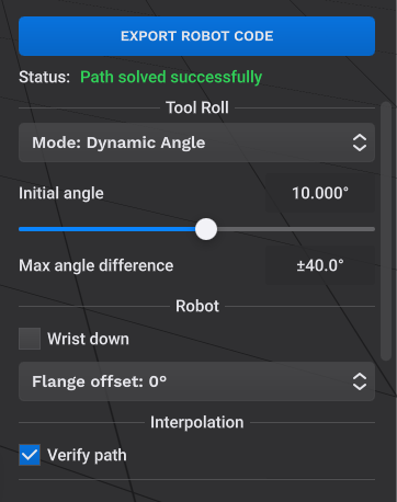
Alternatively, you can select Dynamic Angle with an initial angle of 10 degrees as seen below.
After successfully solving the path with the settings above, the robot movements can be simulated by pressing the play button near the bottom, middle of the screen. The simulation will look like the video below:
The two videos with the different settings are shown below:
Mode: Fixed Angle + Deviation
Mode: Dynamic Angle
cube_5_sides.zip (569 Bytes)